Helix 3D Toolkit – Well Viewer Part 2
In my last post I outlined creation of a 3D well plot with Helix Toolkit. In this post the original code will be refactored to include a two part tubular. The outer tube will represent the well bore, and the inner tube will represent the pipe in the well. Also, we will add a color gradient onto the tubing. Value sets can be mapped to the gradient to show something like temperature or pressures in a well. The refactored code is available in this Github Gist.
The Details
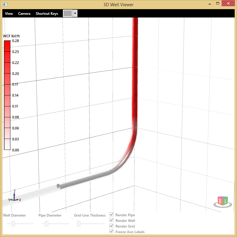
The data plotted in this 3D well viewer comes from a tubing forces torque and drag model. Force values are calculated at regular intervals of depth for tubing in the well. The outer well bore or casing is represented as a transparent glass tube. The pipe inside the well is the mapped gradient of force values (red to white).
Note: there is not a one to one mapping between well profile points and calculated forces. A well profile may be described by 20 or 30 data points describing the centerline of the wellbore. The torque and drag model may return several thousand data points for a length of pipe within the well. The data will need to be interpolated by depth to account for this.
Mapping Values as Texture Coordinates Helix toolkit uses the concept of texture mapping to apply a skin over the 3D objects. If you want to know more about texture mapping its explained in detail on [Wikipedia].
In this example, a linear gradient brush with values ranging from 0 to 1 is used. Values mapped to the brush will need normalized into the range of 0 to 1. Coordinates are given for where to apply the brush values on the geometry. Once a texture coordinates for each 3D point, we can databind them to our 3D plot in XAML
Here is a Github example project that contains all the code.